What is K-Nearest Neighbors (KNN)?

The K-Nearest Neighbor (KNN) algorithm is one of the simplest and most intuitive algorithms in machine learning. Imagine you have a bunch of things (like fruits) and you want to guess which category a new, unknown fruit belongs to. You find the fruits most similar (closest) to this new one and decide what the new fruit is based on what most of its neighbors are.

1. It’s called “non-parametric” because it doesn’t assume anything about the data’s distribution (like linearity, normality, etc.).
2. It’s called “lazy” because it doesn’t train an internal model; it just stores the data and uses it at prediction time.

Getting Started with K-Nearest Neighbors

K-Nearest Neighbors (KNN) is often called a lazy learner because it doesn’t immediately learn a model from the training data. Instead, it stores all the data points and waits until it needs to make a prediction. At the time of classification, it simply calculates the distance between the new data point and all the stored points.

As an example, consider the following table of data points containing two features:

Data Point	Feature 1	Feature 2	Category
A	2.0	2.1	Category 1 (Green Circle)
B	2.5	3.0	Category 1 (Green Circle)
C	5.0	4.0	Category 2 (Orange Triangle)
D	5.5	3.8	Category 2 (Orange Triangle)

Suppose we have a new data point with features (4.7, 3.5), and we need to decide whether it should be Category 1 or Category 2.

KNN Algorithm Working Visualization

Below is a conceptual visualization of how KNN works.

1. Green Circles: Category 1
2. Orange Triangles: Category 2
3. New Point: The unlabeled point (4.7, 3.5)

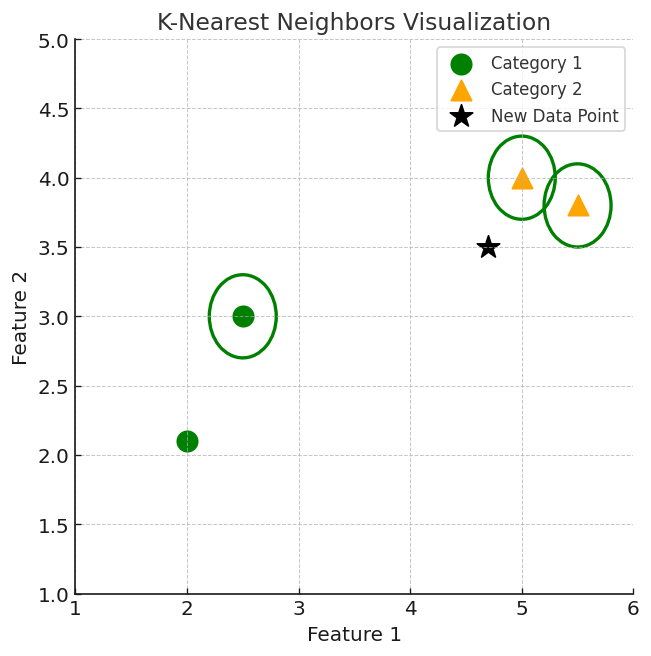
Note: The diagram is not to scale, but it shows Category 1 on the left, Category 2 on the right, and the new point somewhere in the middle.

The new point is classified as Category 2

• Because most of its closest neighbors (e.g., C and D) are orange triangles.
• KNN assigns the category based on the majority vote of these nearby points.

The image shows how KNN predicts the category of a new data point based on its closest neighbours:

1. The green circles represent Category 1.
2. The orange triangles represent Category 2.
3. The new data point checks its closest neighbours—circled in the diagram.
4. Since the majority of its closest neighbours are orange triangles (Category 2), KNN predicts the new data point belongs to Category 2.

In essence, KNN works by measuring proximity (distance) and then using majority voting among the labels of those nearest data points to make a classification decision.

What is ‘K’ in K Nearest Neighbour ?

In K-Nearest Neighbors (KNN), ‘K’ is the number of nearest neighbors we consider when classifying a new data point.

Imagine you move to a new neighborhood and want to make friends. You look around and decide to be friends with the 3 closest people to you. If 2 out of those 3 people like playing football, you might also start playing football. Here, K=3 because you considered your 3 nearest neighbors before making a decision.

Example: Understanding ‘K’ in KNN

Let’s say we have a dataset of fruits based on size and color, and we want to classify a new fruit.

Fruit Name	Size	Color	Category
🍏 Green Apple	Small	Green	Apple
🍏 Green Apple	Medium	Green	Apple
🍌 Banana	Medium	Yellow	Banana
🍌 Banana	Large	Yellow	Banana
❓ Unknown Fruit	Medium	Green	???

We now have a new fruit that is medium in size and green in color. We must decide whether it is an Apple 🍏 or a Banana 🍌.

How K Affects the Decision

1. If K = 1 → Look at only the closest neighbor.
   • The closest fruit is Green Apple 🍏 → The new fruit is classified as Apple.
2. If K = 3 → Look at the 3 nearest neighbors.
   • The three closest neighbors are:
     • 🍏 Green Apple (Medium, Green) → Apple
     • 🍏 Green Apple (Small, Green) → Apple
     • 🍌 Banana (Medium, Yellow) → Banana
   • Majority is 🍏 Apple (2 vs 1) → The new fruit is classified as Apple.
3. If K = 5 → Look at 5 nearest neighbors.
   • The five closest neighbors:
     • 🍏 Green Apple (Medium, Green) → Apple
     • 🍏 Green Apple (Small, Green) → Apple
     • 🍌 Banana (Medium, Yellow) → Banana
     • 🍌 Banana (Large, Yellow) → Banana
   • Tie (2 Apples vs 2 Bananas)!
   • In case of a tie, we might increase K or consider other factors like distance weighting.

Choosing the Right ‘K’

• If K is too small (e.g., K=1) → The decision is very sensitive to one data point, which may be noisy or incorrect.
• If K is too large (e.g., K=100) → The decision becomes too broad and may lose local patterns.
• Best practice: Choose K=3, 5, or sqrt(N) (where N is the number of data points) and test which gives the best results.

Most Popular Distance Metrics Used in KNN

In the K-Nearest Neighbors (KNN) algorithm, the choice of distance metric is crucial as it determines how the “closeness” between data points is measured. Selecting an appropriate distance metric can significantly impact the performance of the KNN classifier. Here are some of the most commonly used distance metrics:

1. Euclidean Distance

This is the most widely used distance metric in KNN and is the default in many libraries, including scikit-learn. It measures the straight-line distance between two points in Euclidean space. It’s suitable for continuous data.

Formula:

$$ d(p,q)=∑i=1n​(pi​−qi​)2​ $$

When to Use:

• When the data is continuous and the scale of features is similar.

2. Manhattan Distance

Also known as “Taxicab” or “City Block” distance, it calculates the sum of the absolute differences between the coordinates of two points.

Formula:

​$$ d(p,q)=∑i=1n∣pi−qi∣d(p, q) = \sum_{i=1}^{n} |p_i – q_i|d(p,q)=∑i=1n​∣pi​−qi​∣​ $$

When to Use:

• When dealing with high-dimensional data.
• When the data contains outliers, as it is less sensitive to them compared to Euclidean distance.

3. Minkowski Distance

This is a generalized form of both Euclidean and Manhattan distances. By adjusting the parameter ppp, it can represent either:

• p = 1: Manhattan Distance
• p = 2: Euclidean Distance

Formula:

$$ d(p,q)=(∑i=1n∣pi−qi∣p)1/pd(p, q) = \left( \sum_{i=1}^{n} |p_i – q_i|^p \right)^{1/p}d(p,q)=(∑i=1n​∣pi​−qi​∣p)1/p $$

When to Use:

• When you want flexibility in choosing the distance metric by tuning the parameter p.

4. Hamming Distance

This metric is used for categorical data and measures the number of positions at which the corresponding elements are different.

Formula:

$$ d(p,q)=∑i=1n[pi≠qi]d(p, q) = \sum_{i=1}^{n} [p_i \neq q_i]d(p,q)=∑i=1n​[pi​=qi​] $$

When to Use:

• When the data is categorical or binary.

 5. Cosine Similarity

Although not a distance metric in the strict mathematical sense, cosine similarity measures the cosine of the angle between two non-zero vectors. It’s particularly useful in text analysis.

Formula:

$$ similarity(A,B)=A⋅B∥A∥∥B∥\text{similarity}(A, B) = \frac{A \cdot B}{\|A\| \|B\|}similarity(A,B)=∥A∥∥B∥A⋅B​ $$

When to Use:

• Commonly used in text mining and information retrieval.
• When the magnitude of the vectors is not as important as their direction.

Working of KNN Algorithm

The K-Nearest Neighbors (KNN) algorithm is a simple, yet powerful, supervised machine learning method used for both classification and regression tasks. It operates on the principle that similar data points are likely to have similar outcomes. Here’s a step-by-step explanation of how KNN works:

Step 1: Select the Number of Neighbors (K)

Choose the number of nearest neighbors to consider when making a prediction. The value of K is crucial; a smaller K can be sensitive to noise, while a larger K may smooth out the decision boundaries too much. Common choices are K=3 or K=5, but the optimal value often depends on the specific dataset.

Step 2: Compute the Distance Between Data Points

Calculate the distance between the new data point (the one to be classified or predicted) and all existing data points in the training set. The Euclidean distance is commonly used for continuous data, calculated as:

$$ d(p,q)=∑i=1n(pi−qi)2d(p, q) = \sqrt{\sum_{i=1}^{n} (p_i – q_i)^2}d(p,q)=∑i=1n​(pi​−qi​)2​ $$

Where p and q are data points, and n is the number of features. Other distance metrics like Manhattan or Minkowski can also be used depending on the data characteristics.

Step 3: Identify the K Nearest Neighbors

Sort all the distances calculated in the previous step in ascending order. Select the top K data points that are closest to the new data point. These are considered its nearest neighbors.

Step 4: Make a Prediction

• For Classification:
  • Each of the K nearest neighbors “votes” for their respective class.
  • The class with the majority vote among the neighbors is assigned to the new data point.
• For Regression:
  • Calculate the average of the target values of the K nearest neighbors.
  • This average is taken as the predicted value for the new data point.

Python Implementation of KNN Algorithm

The K-Nearest Neighbors (KNN) algorithm is a simple yet effective supervised learning algorithm used for classification and regression tasks. Below is a step-by-step Python implementation of KNN using NumPy and Counter from the collections module.

1. Importing Libraries

import numpy as np
from collections import Counter

• NumPy is used for numerical operations, particularly to compute the Euclidean distance.
• Counter (from collections) is used to count the occurrences of elements in an iterable. In KNN, it helps in determining the most common label among the nearest neighbors.

2. Defining the Euclidean Distance Function

def euclidean_distance(point1, point2):
    return np.sqrt(np.sum((np.array(point1) - np.array(point2))**2))

• This function calculates the Euclidean distance between two points in an n-dimensional space.
• The formula used:
  $$ d(p,q)=∑i=1n(pi−qi)2d(p, q) = \sqrt{\sum_{i=1}^{n} (p_i – q_i)^2}d(p,q)=i=1∑n​(pi​−qi​)2​ $$
• It converts the input points into NumPy arrays and computes the squared differences, sums them up, and takes the square root to get the final distance.

3. KNN Prediction Function

def knn_predict(training_data, training_labels, test_point, k):
    distances = []
    
    for i in range(len(training_data)):
        dist = euclidean_distance(test_point, training_data[i])
        distances.append((dist, training_labels[i]))
    
    distances.sort(key=lambda x: x[0])  # Sorting based on distance
    
    k_nearest_labels = [label for _, label in distances[:k]]  # Selecting top K labels
    return Counter(k_nearest_labels).most_common(1)[0][0]  # Most common label

Explanation:

• distances.append(): Stores the computed distance along with the corresponding label from the training data.
• distances.sort(): Sorts the distances in ascending order so that the closest points come first.
• k_nearest_labels: Extracts the labels of the K nearest points.
• Counter(k_nearest_labels).most_common(1)[0][0]: Finds the most frequent label among the K neighbors and returns it as the predicted class.

4. Training Data, Labels, and Test Point

training_data = [[1, 2], [2, 3], [3, 4], [6, 7], [7, 8]]
training_labels = ['A', 'A', 'A', 'B', 'B']
test_point = [4, 5]
k = 3

• The training dataset consists of two classes (‘A’ and ‘B’).
• The test point [4,5] is the new data for which we need to predict the class.
• K = 3, meaning the algorithm will consider the 3 nearest neighbors to make the prediction.

5. Prediction and Output

prediction = knn_predict(training_data, training_labels, test_point, k)
print(prediction)

A

Explanation:

• The algorithm calculates the Euclidean distances of the test point [4,5] to all training points.
• It selects the 3 nearest neighbors.
• Since the majority of these K neighbors belong to class ‘A’, the test point is classified as ‘A’.

Alternative Approach: Using Scikit-Learn

Instead of manually implementing KNN, you can use Scikit-Learn‘s built-in KNeighborsClassifier for an optimized solution.

from sklearn.neighbors import KNeighborsClassifier

knn = KNeighborsClassifier(n_neighbors=3)
knn.fit(training_data, training_labels)
prediction = knn.predict([test_point])

print(prediction[0])

Advantages of Using Scikit-Learn:

✔ Built-in functions for distance calculation and sorting.
✔ Optimized and efficient for large datasets.
✔ Supports hyperparameter tuning and weighting techniques

Applications of the KNN Algorithm

The K-Nearest Neighbors (KNN) algorithm is versatile and widely used across various domains due to its simplicity and effectiveness. Below are some common applications where KNN excels:

1. Image Classification & Recognition

• Use Case: Recognizing handwritten digits or objects in images.
• How KNN Helps:
  • It compares the pixel or feature vectors of a new image to labeled images.
  • Classifies the new image based on the majority label among the closest matches.

2. Recommendation Systems

• Use Case: Movie, music, or product recommendations.
• How KNN Helps:
  • Identifies users with similar preferences (nearest neighbors).
  • Recommends items that these neighbors have liked or purchased.

3. Medical Diagnosis

• Use Case: Classifying patients into disease categories based on symptoms and test results.
• How KNN Helps:
  • Finds patients with similar medical profiles.
  • Predicts the likely diagnosis by majority vote among those similar cases.

4. Fraud Detection

• Use Case: Detecting fraudulent transactions or anomalies in credit card usage.
• How KNN Helps:
  • Compares current transactions to past normal transactions.
  • Flags those that are significantly different as potential fraud.

5. Customer Segmentation

• Use Case: Grouping customers by buying behavior for targeted marketing.
• How KNN Helps:
  • Clusters customers with similar purchasing patterns.
  • Helps businesses tailor promotions and recommendations to each group.

6. Spam Email Filtering

• Use Case: Classifying emails as spam or not spam.
• How KNN Helps:
  • Examines features like word frequency and sender details.
  • Labels an email spam if it closely resembles known spam messages.

7. Intrusion Detection

• Use Case: Cybersecurity and network monitoring.
• How KNN Helps:
  • Compares live network traffic patterns to known normal or malicious traffic.
  • Flags deviations as potential attacks or intrusions.

8. Stock Market & Price Forecasting

• Use Case: Predicting stock prices or housing prices.
• How KNN Helps:
  • Searches for historical data points with similar trends.
  • Uses these data points to forecast short-term movements or property valuations.

Advantages and Disadvantages of the KNN Algorithm

Advantages:

1. Simplicity & Ease of Implementation

• KNN is intuitive: it classifies or predicts based on the closest data points.
• Easy to understand, explain, and implement.

2. No Training Phase (Lazy Learning)

• KNN doesn’t require an explicit training or model-building step.
• Useful when you have frequently updated data; no need to retrain a model repeatedly.

3. Versatile for Classification and Regression

• Works well in multi-class classification tasks.
• Can also be adapted for regression by averaging the labels of nearest neighbors.

4. Adaptable to Different Distance Metrics

• KNN can use Euclidean, Manhattan, or other custom distance measures.
• This flexibility allows it to fit various data types and domains.

5. Intuitive and Easy to Interpret

• The decision boundary is formed by the local neighborhood.
• Predictions can be easily explained by showing the nearest neighbors.

Disadvantages:

1. High Computational Cost

• For a single prediction, KNN must calculate the distance to all data points.
• Not efficient for large datasets; can be slow if many points must be checked.

2. Memory-Intensive

• KNN must store all training data to make predictions.
• Requires significant memory and storage, especially for large datasets.

3. Performance Depends on Feature Scaling

• Distance calculations are sensitive to the scale of features.
• Proper normalization or standardization of features is crucial for good results.

4. Choosing the Right K Value

• A small K can lead to overfitting (noisy decision boundary).
• A large K can lead to underfitting (over-smoothed boundary).
• Finding the optimal K often requires trial and error or cross-validation.

5. Sensitive to Irrelevant or Redundant Features

• All features contribute to distance calculation equally.
• No built-in feature selection means noisy features can distort distances, reducing accuracy.

6. Imbalanced Data Issues

• KNN may bias towards the majority class if the dataset is highly imbalanced.
• The majority class can easily dominate the nearest neighbors.

K-Nearest Neighbor(KNN) Algorithm – FAQs

1. What is the nearest neighbor used for?

Nearest neighbor is used in machine learning and pattern recognition to classify or predict the value of a new data point based on its closest data points. It is commonly applied in:

• Classification: Determining categories (e.g., spam vs. non-spam emails).
• Regression: Predicting values (e.g., house prices based on nearby houses).
• Recommendation Systems: Suggesting products based on user preferences.
• Anomaly Detection: Identifying unusual patterns in data.

---

2. What is the K-nearest neighbor order?

The K-nearest neighbor order refers to the number of closest data points (K) that are considered when making a prediction. The order of neighbors is determined by their distance to the new data point, and KNN ranks them from closest to farthest.

• If K=3, it means the algorithm looks at the 3 nearest neighbors to determine the outcome.
• The choice of K affects the performance:
  • Low K (e.g., K=1) → More sensitive to noise.
  • High K (e.g., K=10) → More generalized decision boundary.

---

3. What is the formula for K-nearest neighbor?

The most commonly used distance formula in KNN is the Euclidean distance, which calculates the straight-line distance between two points in an n-dimensional space: $$ d(p,q)=∑i=1n(pi−qi)2d(p, q) = \sqrt{\sum_{i=1}^{n} (p_i – q_i)^2}d(p,q)=i=1∑n​(pi​−qi​)2​ $$

Where:

• d(p,q)d(p, q)d(p,q) is the distance between points p and q
• pi,qip_i, q_ipi​,qi​ are the feature values of each point
• n is the number of features

Other distance metrics include:

• Manhattan Distance: $$ d(p,q)=∑∣pi−qi∣d(p, q) = \sum |p_i – q_i|d(p,q)=∑∣pi​−qi​∣ $$
• Minkowski Distance (generalized version of Euclidean and Manhattan)
• Hamming Distance (for categorical data)

4. Why is KNN nonparametric?

KNN is nonparametric because:

• It does not assume any specific mathematical form (like linear regression or decision trees).
• It does not require training to estimate parameters. Instead, it memorizes all training data.
• It makes decisions based only on nearby data points at query time, without building an explicit model.
• This makes it highly flexible and able to handle complex and non-linear relationships in data.

However, this also means KNN requires a lot of memory and computation when making predictions.

5. Why is KNN a lazy learner?

KNN is called a lazy learner because:

• It does not build a model during training. Instead, it stores all data points.
• It only performs calculations when a new query is made (i.e., when predicting a new data point).
• It delays all processing until classification or regression is needed, making it computationally expensive at query time.
• Unlike eager learners (e.g., decision trees, neural networks), which build models beforehand, KNN simply searches for the nearest data points when asked.

This makes KNN easy to implement but slow for large datasets.

6. What is the difference between KNN and K-Means?

Feature	KNN (K-Nearest Neighbors)	K-Means (K-Means Clustering)
Type	Supervised Learning	Unsupervised Learning
Purpose	Classification & Regression	Clustering
How it Works	Assigns a label to a new data point based on its nearest K neighbors	Divides data into K clusters without predefined labels
Training?	No explicit training (lazy learner)	Requires training (iterative process)
Example Use	Classifying emails as spam or not	Grouping customers based on purchasing behavior
Distance Metric	Uses Euclidean, Manhattan, etc., to find nearest neighbors	Uses centroid-based clustering

Key takeaway:

• KNN is used for classification and regression (supervised learning).
• K-Means is used for grouping unlabeled data into clusters (unsupervised learning).